Damages caused by earthquakes may be
considered as the result of the geological characteristics of the sites where
they occur. These characteristics are better studied analyzing directly the
ground motions due to the earthquakes. This type of studies, however, is limited
to the areas that present a high level of seismicity [Nakamura, 1989].
To get out of this limitation, systematic analyses of ambient noise were made,
which can be easily performed in areas where the seismicity is low or even
absent [Dikmen & Mirzaoglu, 2005].
The ambient noise shows indeterminable amplitude in time at every moment, being
a stochastic signal resulting by a great number of processes of different
origin (antropic, eolic, oceanic, seismic, etc.) [Bormann, 2002].
On the contrary, it is possible to identify, in frequency, an amplitude oscillation
between a minimum and a maximum [Boashash, 2003].
The knowledge of the ratio between the amplitudes of the horizontal (H) and the vertical (V) components of ambient noise allows
to recognize the natural frequency of the ground vibration (resonance
frequency) [Nakamura, 1989] and to
identify correctly the specific frequencies of oscillation of a building [Sungkono & Triwulan, 2011]. Thus,
the dynamic characteristics of the sites are quickly evaluated without needing
other information [McNamara & Buland, 2004].
In Fig. 1 an example of the trend
of the H/V ratio in frequency is
reported, where the resonance frequency is well identified around 1.4 Hz [Nakamura, 1989].
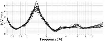
Fig. 1: Trend of H/V ratio as a function of the frequency.
The characterization of the ambient noise amplitude in frequency is essential to evaluate the performances of a seismic network. The amplitude trend, indeed, depends not only on the geology of the observation site and on the characteristic frequencies of the sources producing the noise, but also on the feedback of the acquisition system present at the network. That amplitude is evaluated by the records of the vertical component of the ambient noise at a group of seismic stations, performed on several days having different characteristics (e.g. working days and holidays) [McNamara & Buland, 2004]. On the left side of Fig. 2, records of five minutes of ambient noise are reported, carried out at the Complesso Universitario di Monte S. Angelo of the University of Naples Federico II. The black signal corresponds to the record performed at 4:03 in the night on May 7th 2007, the red one at 10:03 in the morning, the blue one at 16:03 in the afternoon, and the green one at 22:03 in the evening [Lepore et al., 2007]. Instead, on the right side of Fig. 2, different amplitude trends of ambient noise in frequency (between 0.05 and 20 Hz) are reported, distinguished on the basis of the conditions indicated in the legend [Lepore, 2006].

Fig. 2: Amplitude trend of ambient noise in time and frequency.
The definition of the average amplitude of the ambient noise in frequency at a seismic network is very useful to establish the detection level of earthquakes at the same network. For that purpose, it is helpful to make use of models which allow to define the amplitude of simulated earthquakes around a seismic network. That amplitude is calculated using the values of the static stress drop Δσ (difference between the stress values on a fault before and after an earthquake, measured in MPa), the moment magnitude Mw (dimensionless variable which evaluates the earthquake magnitude in terms of energy), and the distance source-receiver r for each simulated earthquake [Boatwright, 1980]. Once determined the amplitude associated with the simulated earthquakes, the acquisition threshold is defined as a specific value of the ratio between that amplitude and the one associated to the ambient noise (SNR, Signal to Noise Ratio, measured in db). The threshold is established on the basis of the overall characteristics of the seismic network and of the amplitude associated to the weakest expected earthquake. All the earthquakes which present a value of that ratio larger than that of the threshold in the previously fixed frequency interval (0.05 ¸ 20 Hz) will be detectable at the seismic network, being distinguished from the ambient noise present at the seismic stations. The values of Δσ, Mw, and r, which identify the first simulated earthquake that exceeds the threshold, define the detection level of the earthquakes at a specific seismic network [Bay, 2003].
In Fig. 3, the trends in frequency of the amplitudes associated with the simulated earthquakes are reported for Mw ranging between 0.5 and 4.5, Δσ equal to 1, 3 and 10 MPa, and r equal to 5 km. For Mw ³ 2.5, it is observed that at a certain frequency (corner frequency) the original amplitude curve is split in three curves on the basis of the Δσ value [Lepore, 2006].

Fig. 3: Amplitude trend associated to simulated earthquakes.
In Fig. 4, the SNR values as a function of frequency are reported calculated starting from the corner frequency, for Mw ranging between 2.0 and 4.5, Δσ equal to 1, 3 and 10 MPa, and r equal to 5 km. Since the threshold was fixed to 6.5 db, it is observed that for Δσ = 1 MPa only the earthquakes with Mw ³ 3.0 exceed the threshold at any frequency, whereas for Δσ = 3 MPa the exceeding already occurs for Mw ³ 2.5. For Δσ equal to 10 MPa, the SNR curve with Mw = 2.0 is not reported, since the corner frequency does not fall anymore (see Fig. 3) in the chosen frequency interval. Therefore, on the basis of what stated before, the minimum detection level of earthquakes is, in this case, Mw = 2.5, for Δσ = 3 MPa and r = 5 km [Lepore, 2006].

Fig. 4: Trend of the Signal to Noise Ratio as a function of frequency.
REFERENCES
Bay F.: "Spectral
shear-wave ground motion scaling in Switzerland", Bull. Seism. Soc. Am.,
93, 414-429, 2003.
Boashash B.:
"Time-Frequency Signal Analysis and Processing", 2003.
Boatwright J.: "A
spectral theory for circular seismic sources", Bull. Seism. Soc. Am.,
70, 1‑27, 1980.
Bormann P.: "New
manual of seismological observatory practice", IASPEI, 2002.
Dikmen U., and Mirzaoglu
M.: "The seismic microzonation map of Yenisehir-Bursa, NW of Turkey, by
means of ambient noise measurements", J. Balkan Geophys. Soc., 8, 53-62,
2005.
Lepore S., Di Fiore V.,
and Rapolla A.: "Features of seismic microtremor signals within a
building", Proceeding of the 26th GNGTS meeting, 13-15 November 2007, Roma.
Lepore S.: "Una
metodologia per la determinazione del livello di detezione di una rete
sismica", Tesi di Laurea, Università degli Studi di Napoli Federico II,
2006.
McNamara D.E., and Buland
R.P.: "Ambient noise levels in the continental United States",
Bull. Seism. Soc. Am. 94, 1517-1527, 2004.
Nakamura Y.: "A
method for dynamic characteristics estimation of subsurface using microtremor
on the ground surface", Q. Rept. Railway Tech. Res. Inst., 30, 25-33,
1989.
Sungkono D.D.W., and
Triwulan W.U.: "Evaluation of buildings strength from microtremor
analyses", Int. J. Civ. Environ. Eng., 11, 108-114, 2011.

